Excel Tip of the Week #393 - AND/OR

What are these functions for? How do they work?

Simple logical tests can be made in Excel with or without the IF function by just writing the two things to be compared either side of a comparison operator, e.g.:

=A1=B1
=C1>D1
=E1<=F1

But sometimes you need to make more sophisticated questions than just a single comparison yes/no. In those cases, the AND and OR functions are what you need. Each lets you complicate logic by considering two or more comparisons, and then providing a single answer depending on a simple, intuitive rule:

AND will be TRUE if ALL the tests are true, and FALSE if ANY are false
OR will be TRUE if ANY of the tests are true, and FALSE if ALL are false

The way you write them is also pretty simple:

=AND(logical test 1, logical test 2, …)
=OR(logical test 1, logical test 2, …)

Note that each and every input has to be a full logical test in its own right. If e.g. comparing several values against a single threshold, it can be tempting to write something like:

=OR(A1, B1, C1)>threshold

…But this doesn’t work. You need to write:

=OR(A1>threshold, B1>threshold, C1>threshold)

Note that you can also combine these two functions by nesting one inside the other. For example, let’s say we want to define items to flag for further investigation as those belonging to transaction class A, and with a value above ±£40,000. If the transaction class is in column A and the transaction amount in B, we can write this as:

=AND(A1=“Class A”, OR(B1>40000, B1<-40000))

The internal OR will calculate first and will be true if the value is either above +40,000 or below -40,000. The result of the OR function is then fed into the next stage, so we check if the item is both in Class A and it meets the OR criteria for size.

More complex situations

If you are using IF – and most of the time a logical value is used, you will be – then often more complex situations can arise where nesting multiple IF inside one another is needed. However, with careful thought and layout, it’s often possible to simplify things. Let’s say we’re dealing with a percentage change calculation. We want to show 0% change if both the current year (A1) and prior year (B1) figures are 0, and an “N/A” value if only the prior value is 0. You could write this with an AND:

=IF(AND(A1=0, B1=0), 0%, IF(B1=0, “N/A”, A1/B1-1)

However, we could also rearrange things to avoid it:

=IF(B1=0, IF(A1=0, 0%, “N/A”), A1/B1-1)

This makes for a shorter and simpler function.

Secondly, it’s also worth thinking about these functions in other contexts. For example, if you’re writing an array function, it’s easy to trip up here. Let’s say we want to create an array formula to find the median value of the items in the A and B categories in this data:

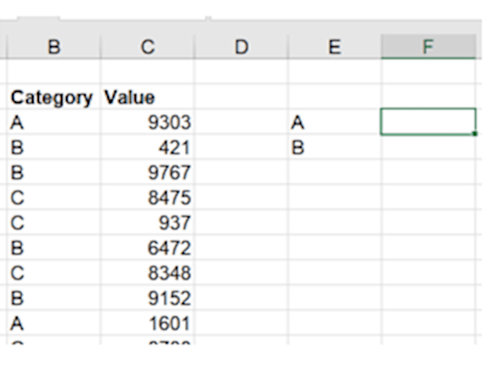
It might be tempting to write:

=MEDIAN(IF(OR(B3:B21=E3, B3:B21=E4), C3:C21, ""))

(pre-Microsoft 365 this sort of formula would need to be confirmed by pressing Ctrl Shift Enter)

The problem here is that, while the two array tests do produce arrays of true/false values, the OR function condenses all of them into a single value – in this case, TRUE – and we just get the median of the entire dataset. Instead, we have to do an equivalent operation without collapsing the array. This takes us to considering how Excel considers true and false values numerically.

In any place where a logical value is expected, Excel will consider a 0 value to be equivalent to FALSE, and any nonzero numerical value to be equivalent to 1. This means we can make equivalents to AND and OR like so:

Multiplying values together will return a nonzero (false) value only if all inputs are nonzero (false), so it works like AND

Adding values will return a zero (true) value only if all inputs are zero (true), so it works like OR

So the correct function for our “MEDIANIF” is:

=MEDIAN(IF((B3:B21=E3) + (B3:B21=E4), C3:C21, ""))

And as a final note, if you’re building measures in Power Pivot, then for whatever reason they use a completely different syntax - && is used as an “and operator”, and || is used as an “or operator”.

• Previous Article - #392 - text to columns redux
• TOTW index
• Next time – The Accessibility Checker